Photo by Nienke van Tellingen on Unsplash

Reference-Based Metagenomic Tax and Func Profiling

Last updated on Sep 9, 2019 10 min read metagenomics

Photo by Nienke van Tellingen on Unsplash

Reference-Based Metagenomic Tax and Func Profiling

Last updated on Sep 9, 2019 10 min read metagenomics

1 Tasks assigned and Questions

Original Publish Date: 9th Sep, 2019

Updated on: 09 September, 2019

This Tutorial mainly Originated form Huttenhower Lab Official Reference and Modified by Tank

1 Tasks assigned and Questions

Questions to deal with

Pipeline Numbered Section and Not to Much Explanation 👌
Library Construction Insert Size of Metagenomic Sequencing 👌(300bp/PE150 Novogene and 350/PE100 BIG)
Some Trimmatic Details 👌(reads were removed adaptor sequences, only trimming and qc)
About Orphan Sequence 👌
How Chocophlan Database Generated 👌

(ChocoPhlAn pangenomes A species’ pangenome is a nonredundant representation of the species’ protein-coding potential Using UCLUST, we then cluster all CDSs from high-quality isolate genomes of a given species at 97% nucleotide identity. One representative (centroid) sequence from each cluster is saved. These centroid sequences constitute the species’ pangenome)

Report Generation with Brief Summary and “what you do with which software and some vital intermediate results” 👌

1.1 Intro To Reference-based Pipeline

This tutorial is set-up to walk you through the process of determining the taxonomic and functional composition of several metagenomic samples. It covers the use of

Metaphlan2 (for taxonomic classification),
HUMAnN2 (for functional classification)

1.2 Requirements

Basic unix skills (there are many tutorials online such as this one)
Tutorial data (commands to download are below)
Full Microbiome Helper Virtual Box Image

1.3 Explore Experimental Design, Sample Sequence Preview and Reference to Map

1.3.1 Experimental Design

The first step in any metagenomics pipeline should be to explore your raw files. For this tutorial there should be a “mapping file”, which contains information about each of the samples called map.txt, along with the sequence data for each sample contained within separate FASTQ files within the directory seq

wc -l map.txt
head map.txt

Table 1.1: metadata design
SampleID	groupID	genotype	compartment	timepoint	replicate	batch	techrep	project	indexnum	pheno	library	longtitute
D6303	drStrMH	MH	R	NA	1	2	2	E	41	stress	4	NA
D6307	drStrMH	MH	R	NA	2	2	2	E	41	stress	4	NA
D6314	drStrMH	MH	R	NA	3	2	2	E	41	stress	4	NA
D6315	drStrMH	MH	R	NA	4	2	2	E	41	stress	4	NA
DWYJ03	drStrWY	WYJ	R	NA	5	2	2	E	41	stress	4	NA
DWYJ11	drStrWY	WYJ	R	NA	6	2	2	E	41	stress	4	NA
DWYJ12	drStrWY	WYJ	R	NA	7	2	2	E	41	stress	4	NA
DWYJ15	drStrWY	WYJ	R	NA	8	2	2	E	41	stress	4	NA
W6306	wetCtrlMH	MH	R	NA	1	2	2	E	41	normal	4	NA
W6308	wetCtrlMH	MH	R	NA	2	2	2	E	41	normal	4	NA
W6312	wetCtrlMH	MH	R	NA	3	2	2	E	41	normal	4	NA
WWYJ08	wetCtrlWY	WYJ	R	NA	4	2	2	E	41	normal	4	NA
WWYJ12	wetCtrlWY	WYJ	R	NA	5	2	2	E	41	normal	4	NA
WWYJ13	wetCtrlWY	WYJ	R	NA	6	2	2	E	41	normal	4	NA

1.3.2 Sample Sequence Summary Statistics Preview with Fastqc

For your own data you may identify outlier samples with low read depth at this stage. It would also be advisable to explore the quality of your data with a tool like FASTQC.

time fastqc -t 12 seq/D6303_1.fq.gz # about 1m30s
time fastqc -t 12 seq/D6303_2.fq.gz # about 1m30s

then we use the multiqc to aggregate results from bioinformatics analyses across many samples into a single report

time multiqc -d seq/ -o result/

see the multiqc aggregated result as belows:multiqc report

for sake of convenience we gunzip the compressed file

gunzip raw_data_example/*gz
wc -l raw_data_example/*.fq ##(stat infor)

1.3.3 Reference Genomes to Map and Indexing-Building

Host Oryza sativa Indica Group and Japonica Group from EnsemblePlants Cultivated rice (O. sativa) and its closest wild relative rice (O. rufipogon)

Note¹

Fist to download the corresponding rice genome

wget -c ftp://ftp.ensemblgenomes.org/pub/plants/release-44/fasta/oryza_sativa/dna/Oryza_sativa.IRGSP-1.0.dna.toplevel.fa.gz
wget -c ftp://ftp.ensemblgenomes.org/pub/plants/release-44/fasta/oryza_indica/dna/Oryza_indica.ASM465v1.dna.toplevel.fa.gz

for sake of convenience, here I only concatenate the Jap and Ind v44 into riceJapIndAggreEnselPlts_v44.fa and its aggregated size 779M

cat Oryza_indica.ASM465v1.dna.toplevel.fa Oryza_sativa.IRGSP-1.0.dna.toplevel.fa > riceJapIndAggreEnselPlts_v44.fa
du -sh riceJapIndAggreEnselPlts_v44.fa

for the downstream mapping with bowtie2 so database indexing as follows:

bowtie2-build riceJapIndAggreEnselPlts_v44.fa ensPltV44  ## 1h

1.4 Pre-processing (Quality Filtering and Host-Originated Removal)

1.4.1 Quality filtering with Trimmomatic and Host-Originated Removal with Bowtie2

Quality filtering and Screening out of Contaminant Reads were performed by Trimmomatic and Bowtie2 which is aggregated by a helpful wrapper kneadData

time (kneaddata -i raw_data_example/D6303_1.fq -i raw_data_example/D6303_2.fq -o kneaddata_out \
-db /mnt/m1/xiaoning/database/rice/ --trimmomatic /conda/share/trimmomatic-0.39-1/ \
-t 4 --trimmomatic-options "SLIDINGWINDOW:4:20 MINLEN:50" \
--bowtie2-options "--very-sensitive --dovetail" --remove-intermediate-output) >>kneaddata.log 2>&1  ## about 24m

you could find the step1 log file

1.4.2 Kneaddata Results Visiualization

You can get a summary of read counts passed at each step broken down by paired and unmatched reads with this command:

kneaddata_read_count_table --input kneaddata_out --output kneaddata_read_counts.txt

library(knitr)
library(ggplot2)
library(reshape2)
mapFile <- read.table("./map.txt",row.names= 1,  header=T, sep="\t")
kneaddata_read_counts <- read.table("./kneaddata_read_counts.txt",row.names= 1,  header=T, sep="\t")
kable(x = kneaddata_read_counts,caption = "kneaddata intermediate result")

Table 1.2: kneaddata intermediate result
	raw.pair1	raw.pair2	trimmed.pair1	trimmed.pair2	trimmed.orphan1	trimmed.orphan2	decontaminated.ensPltV44.pair1	decontaminated.ensPltV44.pair2	decontaminated.ensPltV44.orphan1	decontaminated.ensPltV44.orphan2	final.pair1	final.pair2	final.orphan1	final.orphan2
D6303_1_kneaddata	3333786	3333786	2982355	2982355	176026	93315	1519310	1519310	99593	65778	1519310	1519310	99593	65778

index<- melt(kneaddata_read_counts)

## No id variables; using all as measure variables

p <- ggplot(index, aes(x=variable, y=value,color=variable)) +
  geom_boxplot(alpha=1, outlier.size=0, size=0.7, width=0.4, fill="transparent") +
  geom_jitter(aes(shape=variable), position=position_jitter(0.07), size=1, alpha=0.7) +
  # scale_colour_manual(values=as.character(colors$color)) +
  # scale_shape_manual(values=shapes$shape) +
  labs(x="various intermediated read", y="Counts of read by kneaddata") +
  theme(axis.text.x = element_text(size=10,angle = 90))

p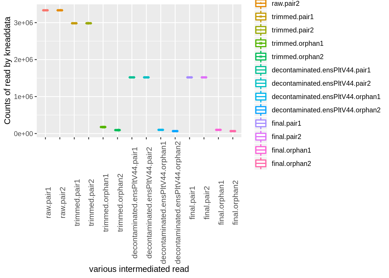

Lastly, We’ll need to move the contaminated sequences and retain read pairs where both forward and reverse reads passed the pre-processing steps

mkdir kneaddata_out/contam_seq

mv kneaddata_out/*_contam_*fastq kneaddata_out/contam_seq
concat_paired_end.pl -p 4 --no_R_match -o cat_reads kneaddata_out/*_paired_*.fastq  ## ? parameter question?

1.5 Taxonomic Profiling with MetaPhlAn2

1.5.1 Metaphlan2 Output

The MetaPhlAn2 output file is the “*bugs_list.tsv” in the temp folder within the output folder. You can take a look at it with less.

Your should see something like this:

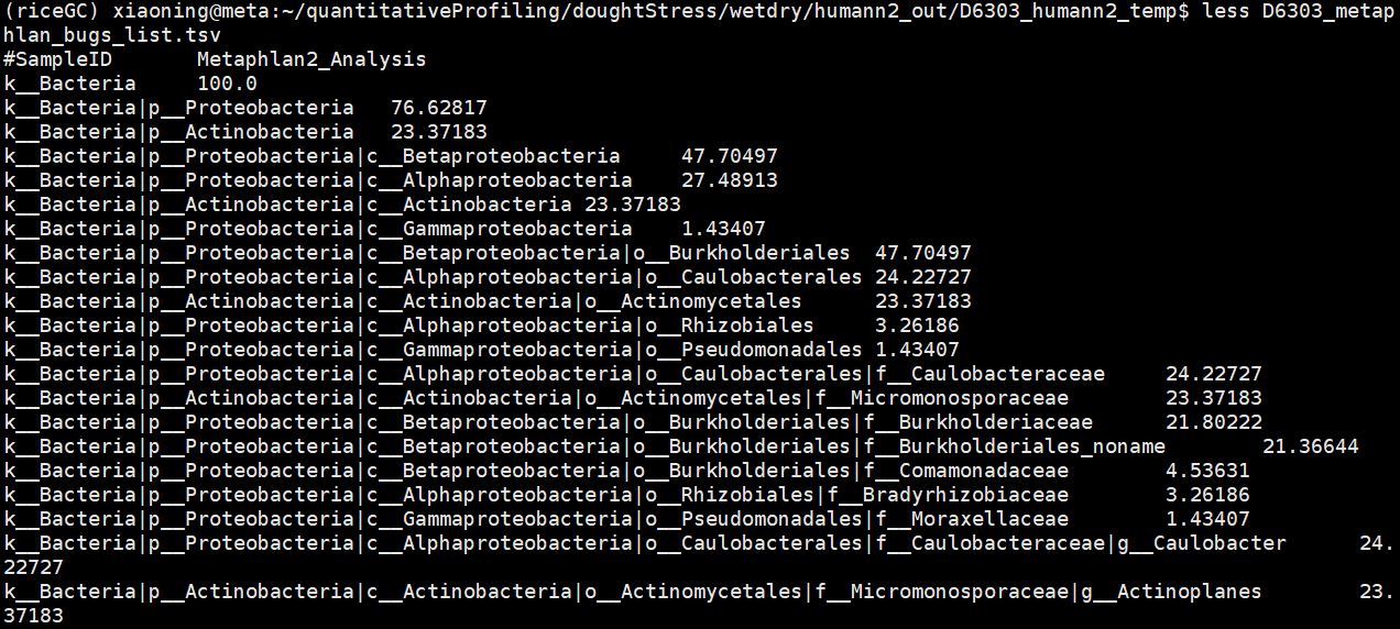
grep 'unclassified'  D6303_metaphlan_bugs_list.tsv

1.5.2 Merging Metaphlan2 Results

We’ve placed all of the MetaPhlAn2 output files in precalculated/metaphlan2_out. All of these files can be merged into one table with this command:

merge_metaphlan_tables.py precalculated/metaphlan2_out/*tsv > metaphlan2_merged.tsv

To plot the taxon heatmap:

metaphlan_hclust_heatmap.py --in metaphlan2_merged.tsv \
            --out metaphlan2_merged_taxonomy_heatmap_top.pdf \
            -c bbcry --top 4 --minv 0.1 -s log

the result with demo as this link pdf

1.6 Functional profiling with HUMAnN and HUMAnN2 Respectively

1.6.1 Running the HUMAnN2 Pipeline (which includes MetaPhlAn2)

1.6.1.1 sigle sample

time (humann2 --threads 8 --input cat_reads/D6303.fastq  --output humann2_out/) >>metaPhlAn_HUMAnN.log 2>&1

1.6.1.2 multiple samples

Running HUMAnN2 on all FASTQs with GNU Parallel

time (parallel -j 1 'humann2 --threads 12 --input {} --output humann2_out/{/.}' ::: cat_reads/*fastq) >>metaPhlAn_HUMAnN_parrel.log 2>&1    ## about 6h* (8 cpu)

Note1²

You should see a logfile of what HUMAnN2 is doing printed

1.7 Code Implementation Log

1.7.1 Software & Corresponding Dependencies, I/O & Database

humann2 v0.11.1
bowtie2 version 2.3
Output files will be written to: /mnt/m1/xiaoning/quantitativeProfiling/doughtStress/wetdry/humann2_out
Writing temp files to directory: /mnt/m1/xiaoning/quantitativeProfiling/doughtStress/wetdry/humann2_out/D6303_humann2_temp
Search mode set to uniref90 because a uniref90 translated search database is selected

1.7.2 Run config settings:

1.7.2.1 DATABASE SETTINGS

nucleotide database folder = /home/meta/db/humann2/chocophlan
protein database folder = /db/humann2/uniref
pathways database file 1 = /conda/lib/python2.7/site-packages/humann2/data/pathways/metacyc_reactions_level4ec_only.uniref.bz2
pathways database file 2 = /conda/lib/python2.7/site-packages/humann2/data/pathways/metacyc_pathways_structured_filtered
utility mapping database folder = /db/humann2/utility_mapping

1.7.2.2 RUN MODES

translated search = diamond
threads = 8

1.7.2.3 SEARCH MODE

search mode = uniref90
identity threshold = 90.0

1.7.2.4 ALIGNMENT SETTINGS

evalue threshold = 1.0
prescreen threshold = 0.01
translated subject coverage threshold = 50.0
translated query coverage threshold = 90.0

1.7.2.5 PATHWAYS SETTINGS

minpath = on
xipe = off
gap fill = on

1.7.2.6 INPUT AND OUTPUT FORMATS

input file format = fastq
output file format = tsv
output max decimals = 10
remove stratified output = False
remove column description output = False
log level = DEBUG

Load pathways database part 1: /conda/lib/python2.7/site-packages/humann2/data/pathways/metacyc_reactions_level4ec_only.uniref.bz2
Load pathways database part 2: /conda/lib/python2.7/site-packages/humann2/data/pathways/metacyc_pathways_structured_filtered

1.7.3 Lay-1 Taxonomic prescreen with metaphlan2

Running metaphlan2.py ……..
Using software: /conda/bin/metaphlan2.py

  /conda/bin/metaphlan2.py /mnt/m1/xiaoning/quantitativeProfiling/doughtStress/wetdry/cat_reads/D6303.fastq \
            -t rel_ab \
            --mpa_pkl /conda/bin/db_v20/mpa_v20_m200.pkl \
            --bowtie2db /conda/bin/db_v20/mpa_v20_m200 \
            -o /mnt/m1/xiaoning/quantitativeProfiling/doughtStress/wetdry/humann2_out/D6303_humann2_temp/D6303_metaphlan_bugs_list.tsv \
            --input_type multifastq \
            --bowtie2out /mnt/m1/xiaoning/quantitativeProfiling/doughtStress/wetdry/humann2_out/D6303_humann2_temp/D6303_metaphlan_bowtie2.txt \
            --nproc 8

Total species selected from prescreen: 9

1.7.4 Lay-2 Pangenome search

1.7.4.1 Creating custom ChocoPhlAn database

Adding file to database: g__Rhodopseudomonas.s__Rhodopseudomonas_palustris.centroids.v0.1.1.ffn.gz
Adding file to database: g__Caulobacter.s__Caulobacter_vibrioides.centroids.v0.1.1.ffn.gz
Creating custom ChocoPhlAn database
Using software: /bin/gunzip

  /bin/gunzip \
  -c /home/meta/db/humann2/chocophlan/g__Rhodopseudomonas.s__Rhodopseudomonas_palustris.centroids.v0.1.1.ffn.gz \
  /home/meta/db/humann2/chocophlan/g__Caulobacter.s__Caulobacter_vibrioides.centroids.v0.1.1.ffn.gz

TIMESTAMP: Completed custom database creation: 1 seconds

1.7.4.2 Bowtie2 index buiding and mapping

Execute command:

  /conda/bin/bowtie2-build \
  -f /mnt/m1/xiaoning/quantitativeProfiling/doughtStress/wetdry/humann2_out/D6303_humann2_temp/D6303_custom_chocophlan_database.ffn \
  /mnt/m1/xiaoning/quantitativeProfiling/doughtStress/wetdry/humann2_out/D6303_humann2_temp/D6303_bowtie2_index

TIMESTAMP: Completed database index : 69 seconds
Nucleotide input file is of type: fastq
Using software: /conda/bin/bowtie2
Remove file: /mnt/m1/xiaoning/quantitativeProfiling/doughtStress/wetdry/humann2_out/D6303_humann2_temp/D6303_bowtie2_aligned.sam
Execute command:

  /conda/bin/bowtie2 \
  -q \
  -x /mnt/m1/xiaoning/quantitativeProfiling/doughtStress/wetdry/humann2_out/D6303_humann2_temp/D6303_bowtie2_index \
  -U /m08/21/2019 11:35:09 PM nt/m1/xiaoning/quantitativeProfiling/doughtStress/wetdry/cat_reads/D6303.fastq \
  -S /mnt/m1/xiaoning/quantitativeProfiling/doughtStress/wetdry/humann2_out/D6303_humann2_temp/D6303_bowtie2_aligned.sam \
  -p 8 \
  --very-sensitive

3038620 reads; of these:0.38% overall alignment rate
TIMESTAMP: Completed nucleotide alignment: 57 seconds
Total nucleotide alignments not included based on small percent identities: 3882
TIMESTAMP: Completed nucleotide alignment post-processing: 85seconds
Total bugs from nucleotide alignment: 2
g__Caulobacter.s__Caulobacter_vibrioides: 2337 hits
g__Rhodopseudomonas.s__Rhodopseudomonas_palustris: 5318 hits
Total gene families from nucleotide alignment: 2018
Unaligned reads after nucleotide alignment: 99.7480764294 %

1.7.5 Lay-3 Translated search running diamond

1.7.5.1 Genefamily abundance with diamond

Remove file: /mnt/m1/xiaoning/quantitativeProfiling/doughtStress/wetdry/humann2_out/D6303_humann2_temp/D6303_diamond_aligned.tsv
Running diamond ……..
Aligning to reference database: uniref90_annotated.1.1.dmnd
Remove file: /mnt/m1/xiaoning/quantitativeProfiling/doughtStress/wetdry/humann2_out/D6303_humann2_temp/tmpSqogM6/diamond_m8_9_XDtR
Using software: /conda/bin/diamond
Execute command:

  /conda/bin/diamond blastx \
  --query /mnt/m1/xiaoning/quantitativeProfiling/doughtStress/wetdry/humann2_out/D6303_humann2_temp/D6303_bowtie2_unaligned.fa\
  --evalue 1.0 \
  --threads 8 \
  --max-target-seqs 20 \
  --outfmt 6 \
  --db /db/humann2/uniref/uniref90_annotated.1.1 \
  --out /mnt/m1/xiaoning/quantitativeProfiling/doughtStress/wetdry/humann2_out/D6303_humann2_temp/tmpSqogM6/diamond_m8_9_XDtR\
  --tmpdir /mnt/m1/xiaoning/quantitativeProfiling/doughtStress/wetdry/humann2_out/D6303_humann2_temp/tmpSqogM6

Execute command:

/bin/cat /mnt/m1/xiaoning/quantitativeProfiling/doughtStress/wetdry/humann2_out/D6303_humann2_temp/tmpSqogM6/diamond_m8_9_XDtR

TIMESTAMP: Completed translated alignment post-processing : 1876 seconds
Total bugs after translated alignment: 3

unclassified: 371720 hits g__Caulobacter.s__Caulobacter_vibrioides: 2337 hits g__Rhodopseudomonas.s__Rhodopseudomonas_palustris: 5318 hits - Total gene families after translated alignment: 24363 - Unaligned reads after translated alignment: 95.8994214479 %

Computing gene families …
humann2.quantify.families - DEBUG: Compute gene families
humann2.store - INFO:

Total gene families : 24363 unclassified : 22494 gene families g__Caulobacter.s__Caulobacter_vibrioides : 827 gene families g__Rhodopseudomonas.s__Rhodopseudomonas_palustris : 1192 gene families

TIMESTAMP: Completed computing gene families : 61 seconds

1.7.5.2 Pathway abundance and coverage

Computing pathways abundance and coverage …
Using python module : /conda/lib/python2.7/site-packages/humann2/quantify/MinPath12hmp.py
Execute command:

  /conda/bin/python /conda/lib/python2.7/site-packages/humann2/quantify/MinPath12hmp.py \
  -any /mnt/m1/xiaoning/quantitativeProfiling/doughtStress/wetdry/humann2_out/D6303_humann2_temp/tmpSqogM6/tmppf6IYQ \
  -map /mnt/m1/xiaoning/quantitativeProfiling/doughtStress/wetdry/humann2_out/D6303_humann2_temp/tmpSqogM6/tmpYsRjNU \
  -report /mnt/m1/xiaoning/quantitativeProfiling/doughtStress/wetdry/humann2_out/D6303_humann2_temp/tmpSqogM6/tmpZGhVL5 \
  -details /mnt/m1/xiaoning/quantitativeProfiling/doughtStress/wetdry/humann2_out/D6303_humann2_temp/tmpSqogM6/tmp69OGKR \
  -mps /mnt/m1/xiaoning/quantitativeProfiling/doughtStress/wetdry/humann2_out/D6303_humann2_temp/tmpSqogM6/tmpyJYmbY
  
  
  /conda/bin/python /conda/lib/python2.7/site-packages/humann2/quantify/MinPath12hmp.py \
  -any /mnt/m1/xiaoning/quantitativeProfiling/doughtStress/wetdry/humann2_out/D6303_humann2_temp/tmpSqogM6/tmpoJMAoh \
  -map /mnt/m1/xiaoning/quantitativeProfiling/doughtStress/wetdry/humann2_out/D6303_humann2_temp/tmpSqogM6/tmpYsRjNU \
  -report /mnt/m1/xiaoning/quantitativeProfiling/doughtStress/wetdry/humann2_out/D6303_humann2_temp/tmpSqogM6/tmpyFEcZF \
  -details /mnt/m1/xiaoning/quantitativeProfiling/doughtStress/wetdry/humann2_out/D6303_humann2_temp/tmpSqogM6/tmpw2N6qI \
  -mps /mnt/m1/xiaoning/quantitativeProfiling/doughtStress/wetdry/humann2_out/D6303_humann2_temp/tmpSqogM6/tmpSkA6Al
  
  /conda/bin/python /conda/lib/python2.7/site-packages/humann2/quantify/MinPath12hmp.py \
  -any /mnt/m1/xiaoning/quantitativeProfiling/doughtStress/wetdry/humann2_out/D6303_humann2_temp/tmpSqogM6/tmp9pjqcS \
  -map /mnt/m1/xiaoning/quantitativeProfiling/doughtStress/wetdry/humann2_out/D6303_humann2_temp/tmpSqogM6/tmpYsRjNU \
  -report /mnt/m1/xiaoning/quantitativeProfiling/doughtStress/wetdry/humann2_out/D6303_humann2_temp/tmpSqogM6/tmpHrs0Bq \
  -details /mnt/m1/xiaoning/quantitativeProfiling/doughtStress/wetdry/humann2_out/D6303_humann2_temp/tmpSqogM6/tmptCq1Vz \
  -mps /mnt/m1/xiaoning/quantitativeProfiling/doughtStress/wetdry/humann2_out/D6303_humann2_temp/tmpSqogM6/tmpq3ERBn
  
  /conda/bin/python /conda/lib/python2.7/site-packages/humann2/quantify/MinPath12hmp.py \
  -any /mnt/m1/xiaoning/quantitativeProfiling/doughtStress/wetdry/humann2_out/D6303_humann2_temp/tmpSqogM6/tmpszWTJj \
  -map /mnt/m1/xiaoning/quantitativeProfiling/doughtStress/wetdry/humann2_out/D6303_humann2_temp/tmpSqogM6/tmpYsRjNU \
  -report /mnt/m1/xiaoning/quantitativeProfiling/doughtStress/wetdry/humann2_out/D6303_humann2_temp/tmpSqogM6/tmpZ45ncK \
  -details /mnt/m1/xiaoning/quantitativeProfiling/doughtStress/wetdry/humann2_out/D6303_humann2_temp/tmpSqogM6/tmpE__fq_ \
  -mps /mnt/m1/xiaoning/quantitativeProfiling/doughtStress/wetdry/humann2_out/D6303_humann2_temp/tmpSqogM6/tmpCQzS3a

Compute pathway abundance for bug: unclassified - Compute pathway abundance for bug: all

TIMESTAMP: Completed computing pathways : 16 seconds

Output files created:

/mnt/m1/xiaoning/quantitativeProfiling/doughtStress/wetdry/humann2_out/D6303_genefamilies.tsv

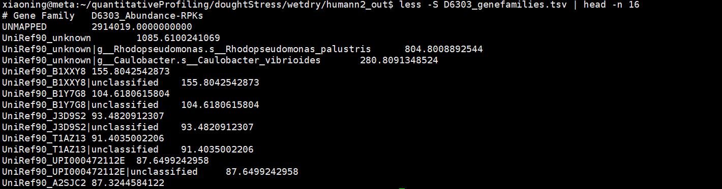
Genefamilies

/mnt/m1/xiaoning/quantitativeProfiling/doughtStress/wetdry/humann2_out/D6303_pathabundance.tsv

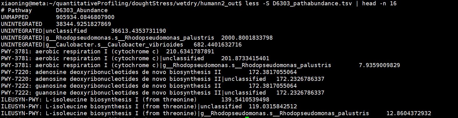
PathwayAbundance

/mnt/m1/xiaoning/quantitativeProfiling/doughtStress/wetdry/humann2_out/D6303_pathcoverage.tsv

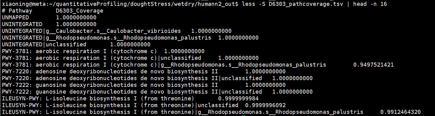
PathwayCoverage

previous studies have found that there are functionally important genes that are absent in the reference Nipponbare genome but present in other rice varieties, indicating that one or a few rice genomes cannot include all of the important genomic content. Hence, to comprehensively capture the genomic diversity in rice, it is necessary to de novo construct the complete genomic sequences for dozens of diverse accessions↩
Setting the option –memory-use maximum will speed up the program if you have enough available memory↩

pipelines

Tank (Xiao-Ning Zhang)

PhD Student @ Data Miner & Coder

I’m a PhD Student majoring in Bioinformatics and Biostatistics who loves computer programming such as C(++), Java, Python and R.